Guide to the data
This is the place to start! Below you will find an introduction to the functionality of the GERLUMPH website, together with examples of how to use the downloaded map data.
Contents
| Map database | The map database is the heart of GERLUMPH, select and download maps and light curves here. |
| Checkout | Finalize your download options and data. |
| Download | Download links to the data. |
| Maps | Map data format and examples. |
| Light curves | Light curve data format and examples. |
| Flux ratios | Flux ratios modelling output format. |
| LSST generator | LSST generator light curve data format. |
| C/C++ | Read binary data in a C/C++ program. |
| Python | Read binary data in a Python program. |
| IDL | Read binary data in a IDL program. |
| PHP | Read binary data in a PHP program. |
Map databasetop »
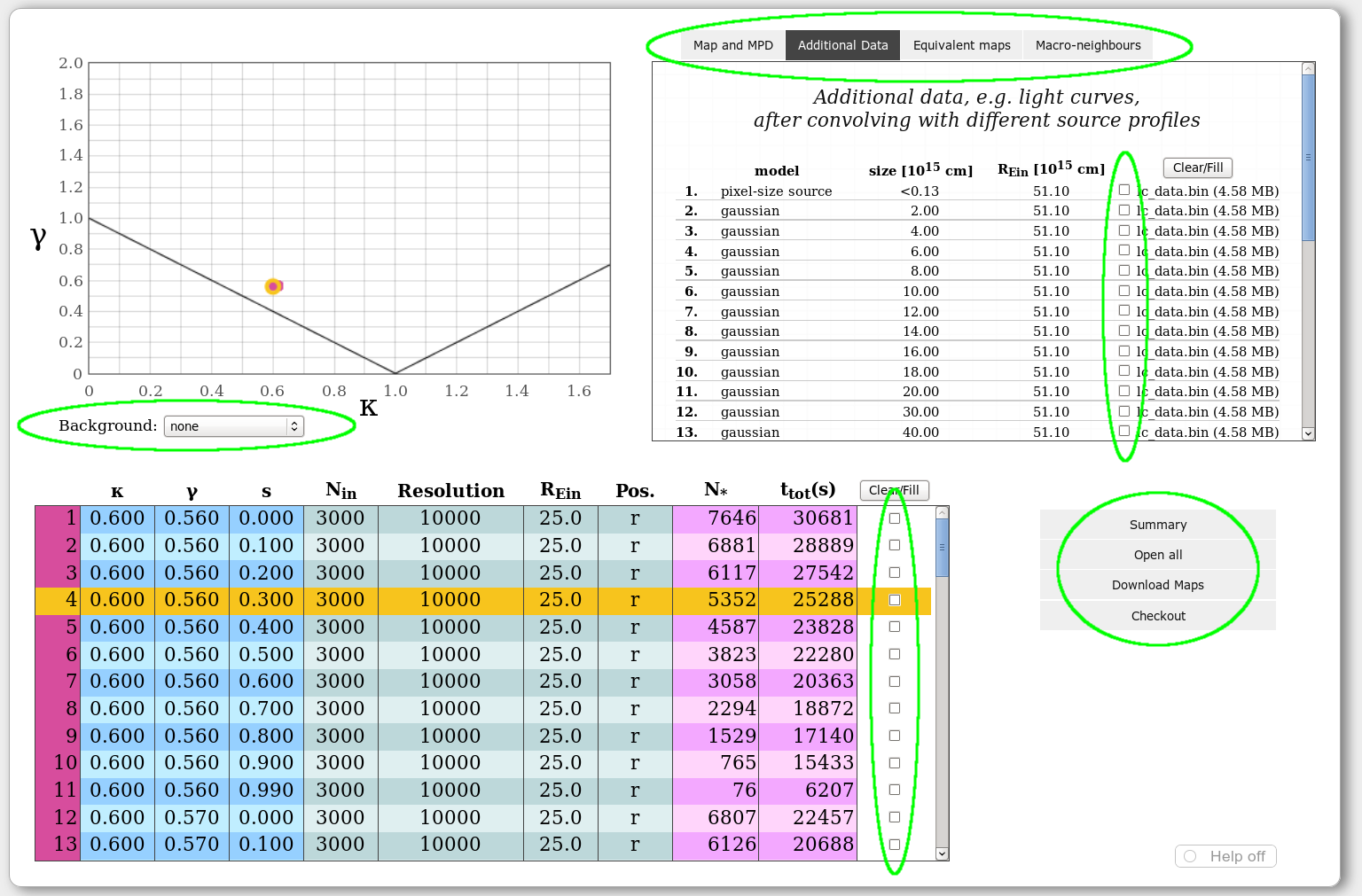
The first step is to set the values of the parameters, as shown in the screenshot:

Select dataset
Select parameters
The matching maps are returned from the database. A number of inspection tools are available:

Tools for single maps
Show various parameter space properties in the background
Select more than one maps
Select additional data
for download
Tools for collections of maps
Checkouttop »
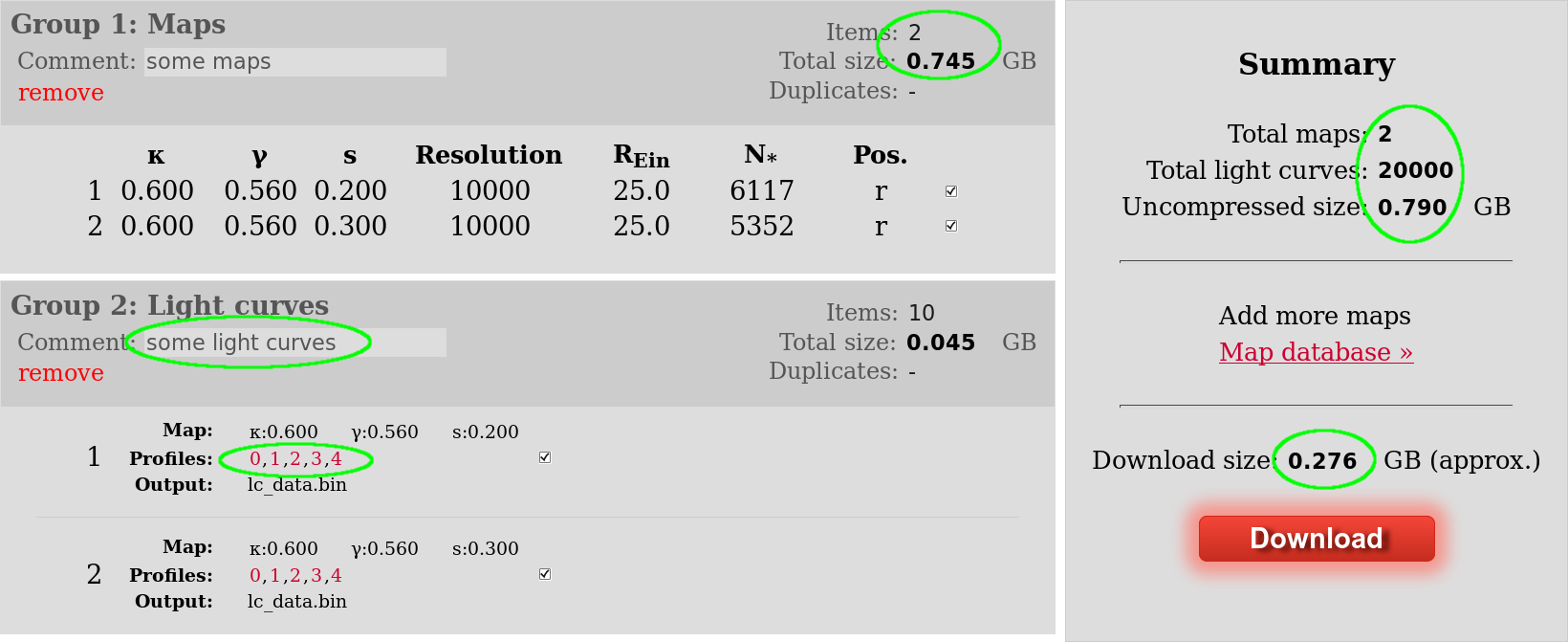
Upon proceeding to checkout, you get a summary of the data you requested for download. Be cautious of duplicate maps and a download-size limit of 10GB.

Number of maps, or convolved maps, in group and size
Total number of maps and light curves
and their final data size
Download size (compressed)
User comment
Profile indices
Next, you will be required to type in a valid email address. After the files are ready for download an email with the donwload links will be sent to you. We delete your email address from our records after sending this email.
Downloadtop »
The download link will take you to a webpage similar to this:

Download links
Download size
Final uncompressed size
Click on the links to start downloading your files. The data format is explained in the next section of this guide.
Map data formattop »
After downloading a group of maps you can extract the files using a command like:
tar -xvf maps_1.tar.bz2
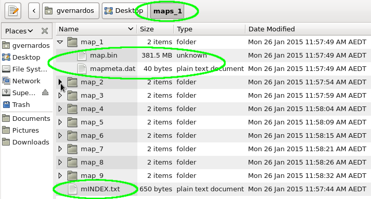
The structure of the extracted directory will be similar to this:

Downloaded data directory
Files for each map
Map reference file
| mINDEX.txt |
This is the reference file to all the downloaded maps: 
| ||
| map.bin |
This is the actual magnification map stored in binary format. The ray counts per pixel are represented in a 4-byte integer format. E.g. you can view the contents of this file by running the shell command: od -t d4 map.bin | head | ||
| mapmeta.dat |
4-line text file containing some metadata about the map, e.g. :
The first two numbers are useful for covnerting the value of each map pixel from ray counts to magnification using the following formula: 
where <μ> is the average magnification, <N> is the average number of rays per pixel, and μij and Nij are the magnification and ray count values respectively, for each map pixel. |
Light curve data formattop »
The process of downloading light curve data is similar to the one for the maps described above, first the files have to be extracted using a command like:
tar -xvf lcurves_1.tar.bz2
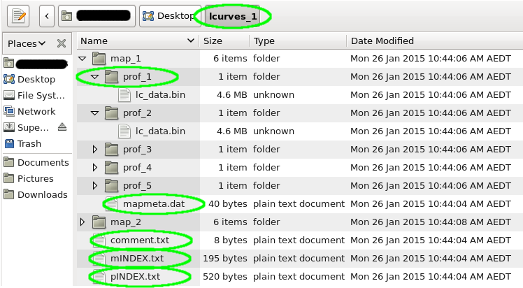
The structure of the extracted directory will be similar to this:

Downloaded data directory
Profiles for each map
Mapmeta for each map
User comment on the data
Map reference file
Profile reference file
| mINDEX.txt |
Same file as the one described in the map section above. |
| pINDEX.txt |
This is the reference file for all the source profiles that were used to generate the light curves: 
|
| lc_data.bin |
This is the actual light curve data stored in binary format. The magnification values are represented by 4-byte floating point numbers. E.g. you can view the contents of this file by running the shell command: od -t d4 lc_data.bin | head |
| mapmeta.dat |
Same file as the one described in the map section above. |
Flux ratio modellingtop »
To be written soon.
LSST light curvestop »
After downloading the light curves you can extract the files using a command like:
tar -xvf output.tar.bz2
The structure of the extracted directory will be similar to this:

The two types of light curves, continuous and sampled, differ only in the sequence of time steps; the former have regular time intervals, of the same length in all bands and for all light curves (thus, different trajectories have different lengths), while the latter have a sequence of time steps distinct for each band but the same for all light curve trajectories. We exploit this and group all the continuous light curves by trajectory and all the sampled ones by band, providing the output in the following files, where X is one of the u,g,r,i,z,y bands:
| X_dates.dat |
One file per band listing time in Modified Julian Date (MJD) and the 5-σ depth of the observation (this is based on the unmicrolensed magnitude of the source in each band and used to calculate the uncertainty in the observed photometry). |
| filter_X_mag.dat |
One file per band with the number of columns matched to the number of dates in the corresponding file above, storing the magnitude values of the sampled light curves in each row. |
| filter_X_dmag.dat |
Same as above for the δmag values. |
| theo_length.dat |
A single file storing the number of time steps, Ni, for each continuous light curve (same in all bands), which have a fixed time interval between them. |
| theo_mag.dat |
A single file with 6 columns, one for each band, and the magnitude values for the continuous light curves stacked vertically, with the first Ni rows corresponding to the first light curve and so on according to the file above. |
| velocities.dat |
A file containing the magnitude and direction of the total velocity of each light curve trajectory, and its υCMB, υ⋆ and υg components in km/s. |
| parameters.json |
A file with the size of the map pixel in physical units and the starting date of the observations in MJD, which is the earliest observation in all of the bands. |
| xy_start_end.dat |
A file containing the starting and ending points (in pixels) of each light curve on the magnification map. |
Using the datatop »
Here are examples of reading binary data in a few popular choices of programming languages. This code is just indicative and can be freely incorporated into user programs and functions. These examples are for reading 4-byte integers in a one- or two-dimensional array. Simple, straightforward, modifications are required to read data in floating point format.
|
|
|
|
|
|
|